Lead Authors: Paul Kushner (University of Toronto) and Elaine Barrow (CCCS/ECCC)
Output from climate models is a distinctive but critical data source for climate analysis and adaptation decision-making; its use in the Canadian North poses a technical challenge to many applications. Climate model output covers historic and future, or ‘projected’, conditions (Eyring et al., 2016). Historic climate model output can be assessed or compared to historic climate data from stations, reanalysis, and other sources. Such a comparison needs to account for climate model experiment design; generally speaking, climate model output cannot be taken as being precisely equal to past observed conditions, for reasons to be discussed below, but it must represent well the statistics of the past climate. A comparison between climate model output and observed historic data can furnish an assessment of climate-model suitability for a given application. If the climate model output is found to be suitable for an application, the model-observation comparison also furnishes numerical adjustments to better align climate model output with regional or local conditions. In applications, this kind of calibration (downscaling) typically targets point/station-level data or gridded data at a finer resolution than the climate model. Projected climate data can then be combined with these adjustments to yield an analysis of future conditions, for a given application.
Climate models represent past, current, and projected climate variability and change in a physically consistent manner. Over several decades, climate model realism has increased alongside improving knowledge of the climate system and advancing computing technology. Basic physical climate models are called GCMs, which stands for global climate models or general circulation models. GCMs comprise complex computer algorithms and software that are based on the principles of fluid dynamics, thermodynamics, and “radiative transfer”, that is, the flow of electromagnetic radiation through the sun-atmosphere-earth system. A GCM represents, on a computer, the mathematical equations of the physical processes of the atmosphere, ocean, cryosphere and land surface, and the interactions and feedbacks between them. The Earth-atmosphere-ocean system is divided into thousands of three-dimensional grid cells, each typically with a horizontal resolution of between 100 and 300 km and containing the mathematical equations describing how energy and materials are transferred through the climate system (Figure 2.2). There are generally between 30 to 40 vertical layers in the atmosphere, three to 10 layers in the soil and between 40 and 50 layers in the ocean.
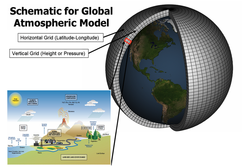
Figure 2.2: Simplified representation of a climate model. The climate processes occurring in each of the many thousands of grid cells are represented by equations based on the fundamental laws of physics, fluid motion and chemistry. [Source: Cannon et al., 2020]
Besides their resolution, GCMs are distinguished by the complexity and completeness of climate system components they represent. Earth System Models (ESMs) represent the most recent generation of climate models. They have all the components of a typical GCM but also include biogeochemical cycles, which describe the transfer of chemicals between living things and their physical and biological environment. ESMs, therefore, can include and explicitly represent the carbon and nitrogen cycles, atmospheric chemistry, ocean ecology and changes in vegetation and land use. Including these biogeochemical cycles means that marine and terrestrial ecosystems (e.g., forests) within the ESM can respond to atmospheric CO2, temperature and rainfall. This allows us to model the fate of carbon from CO2 and other greenhouse gases (GHGs) emitted into the atmosphere through fossil-fuel combustion.
Despite the complexity of climate models, the models are not perfect. Although they represent our best understanding of how the Earth-atmosphere-ocean system works, the climate system is highly complex and it remains fundamentally impossible to model all of its processes. The relatively coarse spatial scales of the models limits explicit modelling of processes that occur at finer-than-grid scales, such as cloud processes, convective processes, and turbulence. In these instances, the physical, chemical and biological processes are parameterized, i.e., their effects are represented by approximations whose design varies across different models.
No climate model exists in a vacuum. The international climate modelling community, which consists of many climate modelling groups running dozens of GCMs and ESMs, organizes itself under the auspices of the Coupled Model Intercomparison Project (CMIP), which is part of the World Climate Research Programme (WCRP). While these climate models are all based on the same physical principles, each group parameterizes the same processes in a slightly different manner, and makes different choices about model structure and horizontal and vertical resolution. In addition, modelling groups make design decisions about which processes to include or not in a given model, which provides another source of model diversity. This results in different models responding in a range of ways to the same forcing, such as anthropogenic GHG forcing. At this point, the present approach to deal with this ‘’uncertainty in model representation of the climate’’ is the pluralist approach that focuses on using ensembles of many climate models (Meeht et al., 2007), selected by various means according to the application [e.g., Massonnet et al., 2012; Evans et al., 2013; Cannon, 2015; Cook et al., 2017; Herger et al., 2018; Docquier and Koenigk, 2021]. However, there are limitations to this approach and alternative approaches have been suggested, as for example the unified approach which focuses more resources on fewer models with finer resolution and improved overall representation of all processes (Hurrell et al., 2009, Palmer, 2012).
As for any mathematical model, climate models need initial conditions as input to initialize the computations and boundary conditions that represent external parameters and variables. Because it is impossible to know the exact state of the climate at one moment in time and because the climate system is a chaotic system (a small difference in initial conditions will result in a new solution – e.g., the timing of oscillations in atmospheric and ocean circulation, like El Niño-Southern Oscillation or the Arctic Oscillation, will differ for each model run with slightly different initial conditions), it is not possible to simulate the time evolution of the climate system in a deterministic way even if the climate model were able to perfectly capture the system. The approach to deal with what is named ‘’ internal climate variability’’ is to run multiple simulations from each model. While an individual simulation or ‘realization’ from one model cannot predict exactly the timing of various phenomena in the climate system, their statistical characteristics can be potentially well characterized by a sufficiently large ensemble of realizations. Consequently, each climate center has submitted to CMIP a multiple number of realizations with the same model. Thus, because of internal climate variability, a model that is run over the historic period is inherently incapable of precisely representing historical day-to-day weather conditions. However, a GCM can be considered to be realistic to the extent that its climate statistics are consistent with observed climate statistics.
Presently, ensembles with multiple realizations of different GCMs and ESMs are used to simulate the pre-industrial climate and the historical evolution of the climate, as well as for creating future climate projections. Given the current complexity of ESMs, an enormous range of climate- and environment-related variables can be output for each ESM grid cell to describe the physical state of the atmosphere, land surface and ocean. Although the actual model simulations are performed typically at time steps of 10-20 minutes, storage considerations mean that data are not archived at such a high time resolution. Instead a tiered approach is employed in which a select few variables are stored on hourly to three hourly timescales and an increasing number of variables are stored on daily and monthly timescales. Model output is in principle available for all the subdomains of interest for this report, including meteorological, snow/hydrology, sea ice and, to a limited extent, permafrost-related variables. However, all model output needs to be evaluated for suitability of the process and spatio-temporal representation depending on the applications.
Climate model results share the same sampling considerations as reanalyses data (Section 2.1.3). Because, as for reanalysis products, GCM/ESM output is gridded, climate model comparison to observations should account for local factors, observational density, and adjustments for specific sites (such as topography not explicitly represented in GCMs).
The enormous and growing amount of model output available presents both challenges and opportunities for applications to the Canadian North. Observational data limitations described in Section 2.1 for the Canadian North suggest that assessment of the realism of GCMs and ESMs remains a serious challenge in this region. Although examples of such applications exist at least on large scales (e.g., Guo and Wang, 2016, Bush and Lemmen, 2019; Mudryk et al., 2021), there are fewer examples of downscaling ESM data for applications of interest to northern communities (e.g., Teufel and Sushama, 2019; Barrette et al., 2020). Finally, finding the best method of selecting among ESMs for suitability of purpose remains a complex issue for the Arctic (e.g., Massonnet et al., 2012). But on balance, given the increased attention to representation of cold climate processes in polar regions, there are now improved opportunities to exploit several generations of ESMs to gauge consistency and robustness of climate projections in the Canadian North.
We provide the following overall guidance that practitioners should keep in mind related to use of climate model output:
- Prior to using climate model outputs in applications for future projections in the Canadian North, a good understanding of how processes are represented in the climate models and a comparison to observed historical climate data should be undertaken. By design, the results of climate models covering the historical period should not be equal to the observations at each instant. Instead, the statistics of climate model outputs should be compared to observed statistics, using multiple realizations of a given climate model, as available.
- Because GCMs and recent ESMs differ in resolution, process representation, etc., it is recommended to use multiple GCMs/ESMs in any given analysis. GCM/ESM selection depends on application.
- Care should be taken when using climate model output to define trends or variability over a long period of time as the effects of internal variability can be significant [Deser et al., 2016], especially at high latitudes; trend analysis requires an assessment over a large ensemble of realizations.
Details about climate model forcing, other aspects of experimental design, the ensembles available for download, discussion of limitations, and consideration of present best practice in applications for the Canadian North are presented in Chapter 4.
References - General description of data sources
Barrette, C., R.D. Brown, R. Way, A. Mailhot, E.P. Diaconescu, P. Grenier, D. Chaumont, D. Dumont, C. Sévigny, S. Howell, and S. Senneville, 2020: Nunavik and Nunatsiavut regional climate information update. In Ropars, P., M. Allard, and M. Lemay (editors). Nunavik and Nunatsiavut: From science to policy, an integrated regional impact study (IRIS) of climate change and modernization, second iteration. ArcticNet, Quebec, Quebec, Canada, 58 pp.
Bush, E. and D.S. Lemmen (editors), 2019: Canada’s Changing Climate Report. Government of Canada, Ottawa, ON. 444 pp.
Cannon, A.L., 2015: Selecting GCM scenarios that span the range of changes in a multimodel ensemble: Application to CMIP5 climate extremes indices. Journal of Climate, 28(3), 1260-1267.
Cannon, A.J., D.I. Jeong, X. Zhang, and F.W. Zwiers, 2020: Climate-Resilient Buildings and Core Public Infrastructure (CRBCPI): An Assessment of the Impact of Climate Change on Climatic Design Data in Canada, Government of Canada, Ottawa, ON. 106 pp.
Cook, L.M., C.J. Anderson, and C. Samaras, 2017: Framework for incorporating downscaled climate output into existing engineering methods: application to precipitation frequency curves. Journal of Infrastructure Systems, 23(4), 04017027, doi: 10.1061/(ASCE)IS.1943-555X.0000382.
Cullather, R.I., T. Hamill, D. Bromwich, X. Wu, and P. Taylor, 2016: Systematic improvements of reanalyses in the Arctic (SIRTA): A White paper. Developed for the Interagency Arctic Research Policy Committee (IARPPC), Accessed on: 2022-02-09. Accessed from: www.iarpccollaborations.org/uploads/cms/documents/sirta-white-paper-final.pdf
Deser, C., L. Terray, and A.S. Phillips, 2016: Forced and internal components of winter air temperature trends over North America during the past 50 years: Mechanisms and implications. Journal of Climate, 29(6), 2237-2258.
Docquier, D. and T. Koenigk, 2021: Observation-based selection of climate models projects Arctic ice-free summers around 2035. Communications Earth & Environment, 2(1), 1-8, doi:10.1038/s43247-021-00214-7.
Evans, J.P., F. Ji, G. Abramowitz, and M. Ekström, 2013: Optimally choosing small ensemble members to produce robust climate simulations. Environmental Research Letters, 8(4), 1-4, doi:10.1088/1748-9326/8/4/044050.
Eyring, V., S. Bony, G.A. Meehl, C.A. Senior, B. Stevens, R.J. Stouffer, and K.E. Taylor, 2016: Overview of the Coupled Model Intercomparison Project Phase 6 (CMIP6) experimental design and organization. Geoscientific Model Development. 9(5), 1937–1958, doi:10.5194/gmd-9-1937-2016.
Guo, D. and H. Wang, 2016: CMIP5 permafrost degradation projection: A comparison among different regions. Journal of Geophysical Research: Atmospheres, 121(9), 4499–4517, doi:10.1002/2015JD024108.
Herger, N., G. Abramowitz, R. Knutti, O. Angélil, K. Lehmann, and B.M. Sanderson, 2018: Selecting a climate model subset to optimise key ensemble properties. Earth System Dynamics, 9(1), 135–151.
Hofstra, N., M.R. Haylock, M. New, P.D. Jones, and C. Frei, 2008: Comparison of six methods for the interpolation of daily European climate data. Journal of Geophysical Research: Atmospheres, 113(D21), doi:10.1029/2008JD010100.
Hofstra, N., M. New, and C. McSweeney, 2010: The influence of interpolation and station network density on the distributions and trends of climate variables in gridded daily data. Climate Dynamics, 35(5), 841–858, doi:10.1007/s00382-009-0698-1.
Hurrell J., G.A. Meehl, D. Bader, T.L. Delworth, B. Kirtman, and B. Wielicki, 2009: A unified modelling approach to climate system prediction. Bulletin of the American Meteorological Society, 90(12), 1819–1832.
Keller, J.D. and S. Wahl, 2021: Representation of Climate in Reanalyses: An Intercomparison for Europe and North America. Journal of Climate, 34(5), 1667-1684.
Kobayashi, S., Y. Ota, Y. Harada, A. Ebita, M. Moriya, H. Onoda, K. Onogi, H. Kamahori, C. Kobayashi, H. Endo, K. Miyaoka, and K. Takahashi, 2015: The JRA-55 Reanalysis: General specifications and basic characteristics. Journal of the Meteorological Society of Japan. Ser. II, 93(1), 5-48, doi:10.2151/jmsj.2015-001.
Massonnet, F., T. Fichefet, H. Goosse, C.M. Bitz, G. Philippon-Berthier, M.M. Holland, and P.-Y. Barriat, 2012: Constraining projections of summer Arctic sea ice. The Cryosphere, 6(6), 1383–1394, doi:10.5194/tc-6-1383-2012.
Meehl, G.A., C. Covey, T. Delworth, M. Latif, B. McAvaney, J.F.B. Mitchell, R.J. Stouffer, and K.E. Taylor, 2007: The WCRP CMIP3 multimodel dataset—a new era in climate change research. Bulletin of the American Meteorological Society, 88(9), 1383-1394.
Mekis, E., N. Donaldson, J. Reid, J. Hoover, A. Zucconi, Q. Li, R. Nitu, and S. Melo, 2018: An Overview of the Surface-Based Precipitation Observations at Environment and Climate Change Canada. Atmosphere-Ocean, 56(2), 71-95. doi:10.1080/07055900.2018.1433627.
Mekis, E., and W.D. Hogg, 1999: Rehabilitation and analysis of Canadian daily precipitation time series. Atmosphere-Ocean, 37(1), 53–85. doi:10.1080/07055900.1999.9649621.
Mekis, É. and L.A. Vincent, 2011: An overview of the second generation adjusted daily precipitation dataset for trend analysis in Canada. Atmosphere-Ocean, 49(2), 163-177.
Mudryk, L.R., J. Dawson, S.E. Howell, C. Derksen, T.A. Zagon, and M. Brady, 2021: Impact of 1, 2 and 4 °C of global warming on ship navigation in the Canadian Arctic. Nature Climate Change, 11(8), 673-679, doi:10.1038/s41558-021-01087-6.
Palmer, T., 2012: Towards the probabilistic earth-system simulator: a vision for the future of climate and weather prediction. Quarterly Journal of the Royal Meteorological Society, 138(665), 841-861.
Przybylak, R. and P. Wyszyński, 2020. Air temperature changes in the Arctic in the period 1951–2015 in the light of observational and reanalysis data. Theoretical and Applied Climatology, 139(1), 75-94, doi: 10.1007/s00704-019-02952-3.
Serreze, M.C. and R.G. Barry, 2014: The Arctic climate system, 2nd edn., Cambridge University Press, Cambridge, 415 pp.
Teufel, B. and L. Sushama, 2019: Abrupt changes across the Arctic permafrost region endanger northern development. Nature Climate Change, 9(11), 858–862.
Vincent, L.A., M.M. Hartwell, and W.L. Wang, 2020: A third generation of homogenized temperature for trend analysis and monitoring changes in Canada’s climate. Atmosphere-Ocean, 58(3), 173-191, doi:10.1080/07055900.2020.1765728.
Vincent, L.A., X.L. Wang, E.J. Milewska, H. Wan, F. Yang, and V. Swail, 2012: A second generation of homogenized Canadian monthly surface air temperature for climate trend analysis, Journal of Geophysical Research: Atmospheres, 117(D18), doi:10.1029/2012JD017859.